- Tham gia
- 3/7/07
- Bài viết
- 4,946
- Được thích
- 23,213
- Nghề nghiệp
- Dạy đàn piano
Phỏng dịch từ cuốn Formulas and Functions with Microsoft Office Excel 2007 của Paul McFedries
Part II: HARNESSING THE POWER OF FUNCTIONS - Tận dụng sức mạnh của các hàm
PART II - HARNESSING THE POWER OF FUNCTIONS
Phần II - Tận dụng sức mạnh của các hàm
Chapter 12 - WORKING WITH STATISTICAL FUNCTIONS
Chương 12 - Làm việc với các hàm thống kê
12.1. Understanding Descriptive Statistics
Tìm hiểu về thống kê mô tả
Trong chương này, do hầu hết các hàm tôi đã trình bày chi tiết ở topic: Các hàm Thống kê, nên tôi sẽ không trình bày lại danh sách các hàm, cú pháp và chú giải các đối số của mỗi hàm nữa (không theo như nguyên bản cuốn sách này). Trong các bài dịch sau đây, khi nói đến một hàm nào, tôi sẽ tạo liên kết (link) đến bài viết về hàm đó. Nếu muốn tìm hiểu kỹ hơn về cú pháp và cách sử dụng các đối số (argument), các bạn theo những liên kết này để xem.
Part II: HARNESSING THE POWER OF FUNCTIONS - Tận dụng sức mạnh của các hàm
- Chapter 6: Understanding Functions - Tìm hiểu các hàm
- Chapter 7: Working with Text Functions - Làm việc với các hàm xử lý chuỗi văn bản
- Chapter 8: Working with Logical and Information Functions - Làm việc với các hàm luận lý và tra cứu thông tin
- Chapter 9: Working with Lookup Functionshttp://www.giaiphapexcel.com/forum/showthread.php?t=11284 - Làm việc với các hàm tìm kiếm
- Chapter 10: Working with Date and Time Functionshttp://www.giaiphapexcel.com/forum/showthread.php?t=11365 - Làm việc với các hàm ngày tháng và thời gian
- Chapter 11: Working with Math Functionshttp://www.giaiphapexcel.com/forum/showthread.php?t=11551 - Làm việc với các hàm toán học
- Chapter 12: Working with Statistical Functionshttp://www.giaiphapexcel.com/forum/showthread.php?t=11623 - Làm việc với các hàm thống kê
PART II - HARNESSING THE POWER OF FUNCTIONS
Phần II - Tận dụng sức mạnh của các hàm
Chapter 12 - WORKING WITH STATISTICAL FUNCTIONS
Chương 12 - Làm việc với các hàm thống kê
Excel’s statistical functions calculate all the standard statistical measures, such as average, maximum, minimum, and standard deviation. For most of the statistical functions, you supply a list of values (which could be an entire population or just a sample from a population). You can enter individual values or cells, or you can specify a range. Excel has dozens of statistical functions, many of which are
rarely, if ever, used in business.
Những hàm thống kê của Excel tính toán tất cả những các số đo thống kê chuẩn như trung bình, lớn nhất, nhỏ nhất, và độ lệch chuẩn. Đối với hầu hết các hàm thống kê, bạn cung cấp cho nó một danh sách các giá trị (có thể là toàn bộ tập hợp hay chỉ là một mẫu của tập hợp). Bạn có thể nhập những giá trị hoặc những ô riêng lẻ, hay là xác định một mảng. Excel có hàng chục hàm thống kê, có nhiều hàm trong số đó hiếm khi được sử dụng trong công việc kinh doanh.
12.1. Understanding Descriptive Statistics
Tìm hiểu về thống kê mô tả
One of the goals of this book is to show you how to use formulas and functions to turn a jumble of numbers and values into results and summaries that give you useful information about the data. Excel’s statistical functions are particularly useful for extracting analytical sense out of data nonsense. Many of these functions might seem strange and obscure, but they reward a bit of patience and effort with striking new views of your data.
Một trong những mục đích của cuốn sách này là trình bày cho bạn cách sử dụng các công thức và các hàm để biến một mớ hỗn độn những con số và những giá trị thành những kết quả và bảng tổng kết, nhằm cho bạn thông tin hữu dụng về dữ liệu. Các hàm thống kê của Excel đặc biệt hữu dụng cho việc trích xuất ra những phân tích có nghĩa khỏi những dữ liệu vô nghĩa. Nhiều hàm trong số này có vẻ lạ lẫm và khó hiểu, nhưng chúng sẽ đền đáp cho sự kiên nhẫn và nỗ lực của bạn bằng những cái nhìn mới đáng ngạc nhiên cho dữ liệu.
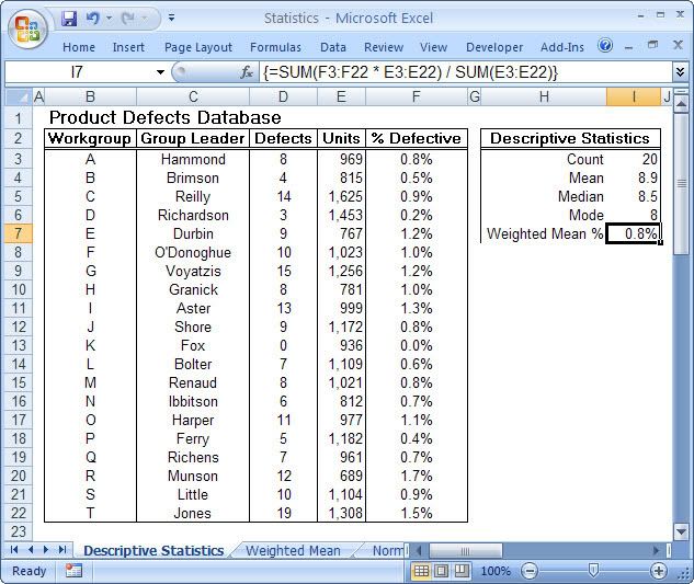
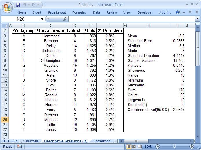
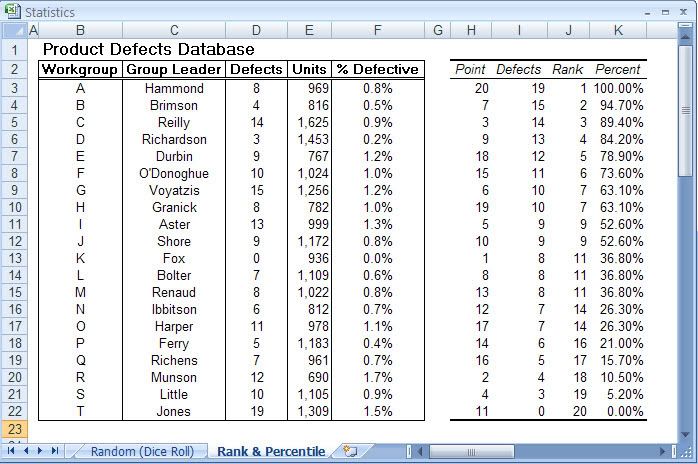
This is particularly true of the branch of statistics known casually as descriptive statistics (or summary statistics). As the name implies, descriptive statistics are used to describe various aspects of a data set, to give you a better overall picture of the phenomenon underlying the numbers. In Excel’s statistical repertoire, 16 measures make up its descriptive statistics package: sum, count, mean, median, mode, maximum, minimum, rank, kth largest, kth smallest, standard deviation, variance, standard error of the mean, confidence level, kurtosis, and skewness.
Điều này đặc biệt đúng với nhóm thống kê được biết với tên là thống kê mô tả (hay thống kê tổng hợp). Như tên gọi của nó, thống kê mô tả được sử dụng để mô tả những khía cạnh khác nhau của một tập hợp dữ liệu, nhằm mang lại cho bạn một cái nhìn rõ ràng hơn về sự thật ở bên dưới các con số. Trong kho thống kê của Excel, có 16 số đo thống kê tạo nên một gói thống kê mô tả: sum (tính tổng), count (đếm), mean (giá trị trung bình), median (trung bình vị), mode (số lần xuất hiện), maximum (giá trị lớn nhất), minimum (giá trị nhỏ nhất), rank (thứ hạng), kth largest (giá trị lớn thứ k), kth smallest (giá trị nhỏ thứ k), standard deviation (độ lệch chuẩn), variance (phương sai), và những lỗi thông thường của giá trị trung bình, mức tin cậy, độ nhọn, hệ số lệch...
In this chapter, you’ll learn how to wield all of these statistical measures (except sum, which you’ve already seen earlier in this book).
Trong chương này, bạn sẽ học cách nắm vững tất cả các số đo thống kê (ngoại trừ sum(tính tổng) bạn đã học trong phần trước).
Một trong những mục đích của cuốn sách này là trình bày cho bạn cách sử dụng các công thức và các hàm để biến một mớ hỗn độn những con số và những giá trị thành những kết quả và bảng tổng kết, nhằm cho bạn thông tin hữu dụng về dữ liệu. Các hàm thống kê của Excel đặc biệt hữu dụng cho việc trích xuất ra những phân tích có nghĩa khỏi những dữ liệu vô nghĩa. Nhiều hàm trong số này có vẻ lạ lẫm và khó hiểu, nhưng chúng sẽ đền đáp cho sự kiên nhẫn và nỗ lực của bạn bằng những cái nhìn mới đáng ngạc nhiên cho dữ liệu.
This is particularly true of the branch of statistics known casually as descriptive statistics (or summary statistics). As the name implies, descriptive statistics are used to describe various aspects of a data set, to give you a better overall picture of the phenomenon underlying the numbers. In Excel’s statistical repertoire, 16 measures make up its descriptive statistics package: sum, count, mean, median, mode, maximum, minimum, rank, kth largest, kth smallest, standard deviation, variance, standard error of the mean, confidence level, kurtosis, and skewness.
Điều này đặc biệt đúng với nhóm thống kê được biết với tên là thống kê mô tả (hay thống kê tổng hợp). Như tên gọi của nó, thống kê mô tả được sử dụng để mô tả những khía cạnh khác nhau của một tập hợp dữ liệu, nhằm mang lại cho bạn một cái nhìn rõ ràng hơn về sự thật ở bên dưới các con số. Trong kho thống kê của Excel, có 16 số đo thống kê tạo nên một gói thống kê mô tả: sum (tính tổng), count (đếm), mean (giá trị trung bình), median (trung bình vị), mode (số lần xuất hiện), maximum (giá trị lớn nhất), minimum (giá trị nhỏ nhất), rank (thứ hạng), kth largest (giá trị lớn thứ k), kth smallest (giá trị nhỏ thứ k), standard deviation (độ lệch chuẩn), variance (phương sai), và những lỗi thông thường của giá trị trung bình, mức tin cậy, độ nhọn, hệ số lệch...
In this chapter, you’ll learn how to wield all of these statistical measures (except sum, which you’ve already seen earlier in this book).
Trong chương này, bạn sẽ học cách nắm vững tất cả các số đo thống kê (ngoại trừ sum(tính tổng) bạn đã học trong phần trước).
You can download the workbook that contains this chapter’s examples here:
Bạn có thể tải về bảng tính với những ví dụ trong chương này tại đây:
Trong chương này, do hầu hết các hàm tôi đã trình bày chi tiết ở topic: Các hàm Thống kê, nên tôi sẽ không trình bày lại danh sách các hàm, cú pháp và chú giải các đối số của mỗi hàm nữa (không theo như nguyên bản cuốn sách này). Trong các bài dịch sau đây, khi nói đến một hàm nào, tôi sẽ tạo liên kết (link) đến bài viết về hàm đó. Nếu muốn tìm hiểu kỹ hơn về cú pháp và cách sử dụng các đối số (argument), các bạn theo những liên kết này để xem.
Lần chỉnh sửa cuối:
 22)
22)